Chapter 6 Estimation

Introduction

Statistical inference

• Estimation: estimating the values of specific population parameters.
• Hypothesis testing: testing whether the value of a population parameter is equal to some specific value.

Estimation

• Point estimation: obtaining specific values as estimates of parameters.
• Interval estimation: specifying a range within which the parameter values are likely to fall.

Random sample

• A random sample is a selection of some members of the population such that each member is independently chosen and has a known nonzero probability of being selected.
• A simple random sample is a random sample in which each group member has the same probability of being selected. For ease of discussion, we use the abbreviated term “random sample” to denote a simple random sample.

Sampling distribution

The sampling distribution of a statistic is the distribution of values of that statistic (like sample mean or median), computed from all possible samples of size $n$ randomly selected from the same reference population.

Construction of a sampling distribution

1. From a population of size $N$, randomly select from all possible samples of size $n$.
2. Compute the statistic of interest for each sample.
3. Create a frequency distribution of the statistic.

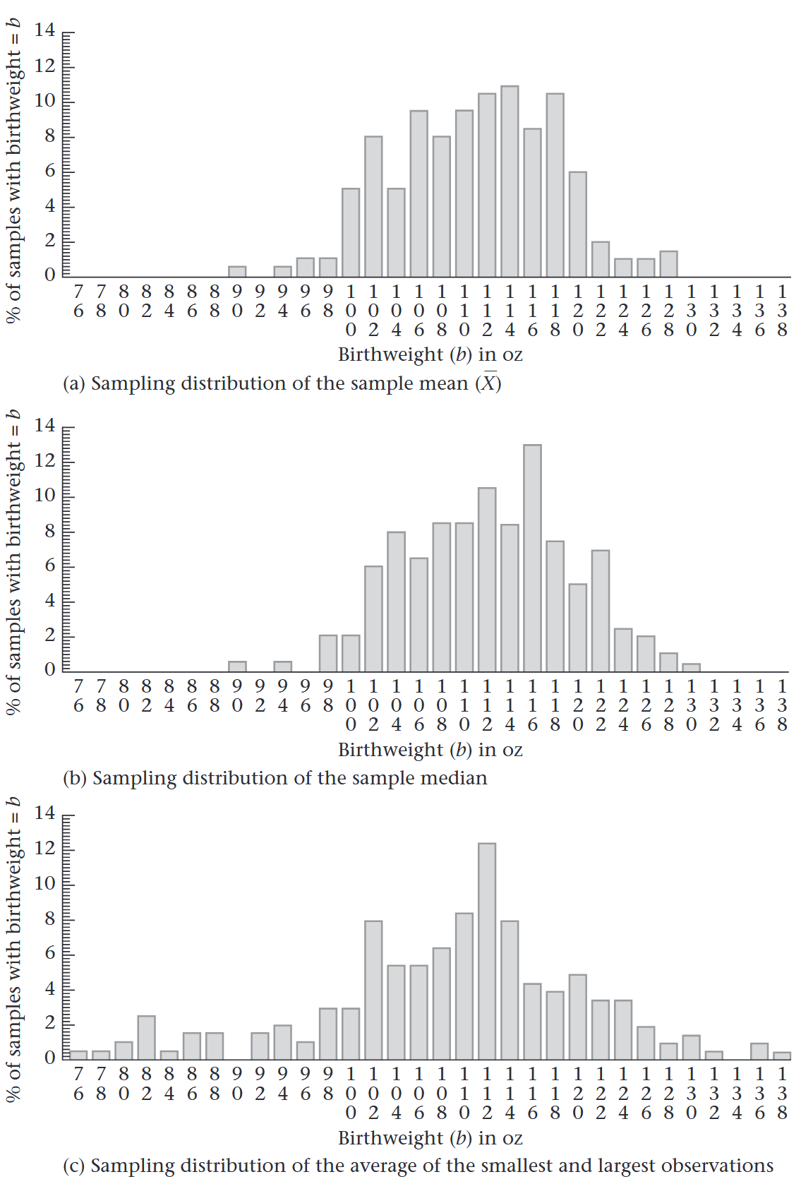
Example: Sampling distributions of sample mean/median/average of smallest and largest for 200 random samples of size 10 selected from the population of 1000 birthweights (100 = 100.0–101.9, etc.). Frequency distributions of of sample mean/median/average of smallest and largest are showing below.

Estimation of the Mean of a Distribution

Let $X_1, \dots, X_n$ be a random sample from a population with mean $\mu$. A natural estimator to use for estimating the population mean $\mu$ is the sample mean:

$$\bar{X} = \frac{1}{n} \sum_{i=1}^{n} X_i,$$

which means:

$$E(\bar{X}) = \mu.$$

• The above equation holds for any population regardless of its underlying distribution. In words, we refer to $\bar{X}$ as an unbiased estimator of $\mu$.
• $\bar{x}$ is a single realization of a random variable $\bar{X}$ over all possible samples of size $n$ that could have been selected from the population.
• In the rest of this text, the symbol $X$ denotes a random variable, and $x$ denotes a specific realization of the random variable $X$ in a sample.

Why is $\bar{X}$ chosen rather than any of the other unbiased estimators? The reason is that if the underlying distribution of the population is normal, then it can be shown that the unbiased estimator with the smallest variance is given by $\bar{X}$. Thus $\bar{X}$ is called the minimum variance unbiased estimator of $\mu$.

Standard error of the sample mean

Why then is it preferable to estimate parameters from large samples rather than from small ones? The intuitive reason is that the larger the sample size, the more precise an estimator $\bar{X}$ is.

Let $X_1, \dots, X_n$ be a random sample from a population with variance $\sigma^2$.

$$\text{Var}(\bar{X}) = \frac{1}{n^2} \text{Var}\left(\sum_{i=1}^{n} X_i\right) = \frac{1}{n^2} \sum_{i=1}^{n} \text{Var}(X_i)$$

Since $\text{Var}(X_i) = \sigma^2$,

$$\text{Var}(\bar{X}) = \frac{1}{n^2}(\sigma^2 + \sigma^2 + \cdots + \sigma^2) = \frac{1}{n^2}(n\sigma^2) = \frac{\sigma^2}{n}$$

$$sd(\bar{X}) = \frac{\sigma}{\sqrt{n}}$$

This is the standard error of the mean (sem) or standard error (se). The standard error is a quantitative measure of the variability of sample mean.

In practice, the population variance $\sigma^2$ is rarely known. A reasonable estimator for the population variance $\sigma^2$ is the sample variance $s^2$, thus the standard error could be estimated by $s/\sqrt n$.

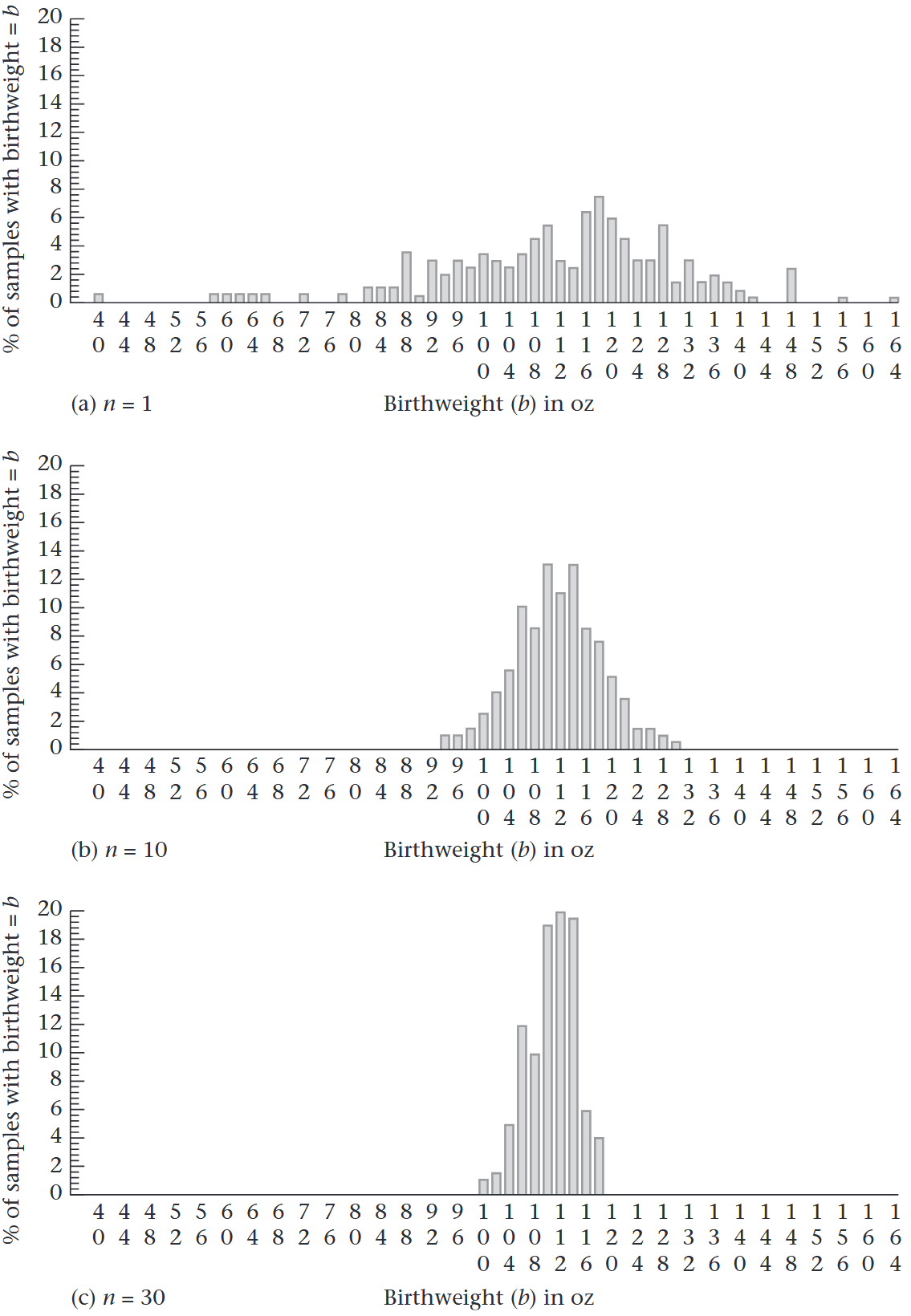
Example: Illustration of the standard error of the mean (100 = 100.0–103.9, etc.) The frequency distribution of the sample mean is plotted for 200 samples of size 1/10/30.

The spread of the frequency distribution: $n=1 > n=10 > n=30$.

Central-Limit Theorem and Interval Estimation

Let $X_1, \dots, X_n$ be a random sample from some population with mean $\mu$ and variance $\sigma^2$. Then for large $n$,

$$\bar{X} \dot{\sim} N\left(\mu, \frac{\sigma^2}{n}\right)$$

even if the underlying distribution of individual observations is not normal. ($\dot{\sim}$ means "approximately distributed.")

Interval estimation: if $\mu$ and $\sigma^2$ were known, A $100\% \times (1 - \alpha)$ CI is:

$$\left( \bar{x} - z_{1-\alpha/2} \cdot \frac{s}{\sqrt{n}},\ \bar{x} + z_{1-\alpha/2} \cdot \frac{s}{\sqrt{n}} \right)$$

This is because:

$$Z = \frac{\bar{X} - \mu}{\sigma / \sqrt{n}}$$

$Z$ follows a standard normal distribution; 95% of $Z$ values fall between $-1.96$ and $+1.96$ (the 2.5th and 97.5th percentiles). 95% of all such sample means will fall within the interval $(\mu - 1.96\ \sigma / \sqrt n), (\mu + 1.96\ \sigma / \sqrt n)$. This assumes $\sigma$ is known, which is rarely true in practice.

$t$ Distribution

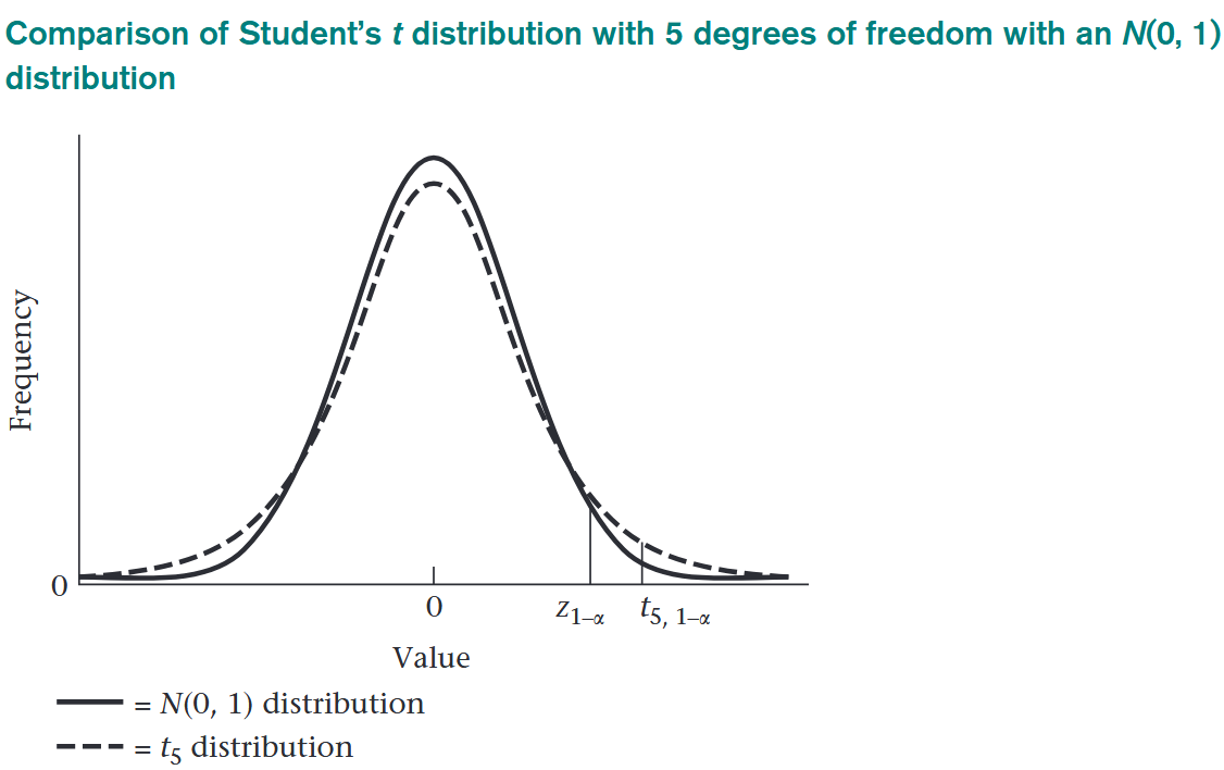
Distribution of sample mean with unknown $\sigma$: If $X_1, \dots, X_n \sim N(\mu, \sigma^2)$ and are independent, then

$$\frac{\bar{X} - \mu}{S / \sqrt{n}} \sim t_{n-1}$$

is distributed as a $t$ distribution with $(n - 1) df$ (degrees of freedom). The $t$ distribution with $d$ degrees of freedom is sometimes referred to as the $t_d$ distribution.

NOTE: $S$ means random variable of sample standard deviation.

The $100 \times u$th percentile of a $t$ distribution with $d$ degrees of freedom is denoted by $t_{d,u}$, that is,

$$P(t_d < t_{d,u}) \equiv u$$

The difference between the $t$ distribution and the normal distribution is greatest for small values of $n$ ($n$ < 30).

Confidence Interval for the Mean of a Normal Distribution

A $100\% \times (1 - \alpha)$ CI for the mean $\mu$ of a normal distribution with unknown variance is

$$\left( \bar{x} - t_{n-1,\, 1-\alpha/2} \cdot \frac{s}{\sqrt{n}},\ \bar{x} + t_{n-1,\, 1-\alpha/2} \cdot \frac{s}{\sqrt{n}} \right)$$

Shorthand: $\bar{x} \pm t_{n-1,\, 1-\alpha/2} \cdot s/\sqrt{n}$.

Derivation: start from

$$P\left(t_{n-1,\, \alpha/2} < \frac{\bar{X} - \mu}{S/\sqrt{n}} < t_{n-1,\, 1-\alpha/2}\right) = 1 - \alpha$$

By symmetry of the $t$ distribution, $t_{n-1,\, \alpha/2} = -t_{n-1,\, 1-\alpha/2}$, so

$$P\left(\bar{X} - t_{n-1,\, 1-\alpha/2} \cdot \frac{S}{\sqrt{n}} < \mu < \bar{X} + t_{n-1,\, 1-\alpha/2} \cdot \frac{S}{\sqrt{n}}\right) = 1 - \alpha$$

NOTE:

• $S$ denotes the sample standard deviation as a random variable; $s$ is its observed value.
• $X_1, \dots, X_n$ should be normal distribution.

Confidence Interval for the Mean (Large-Sample Case)

Equation 6.7: An approximate $100\% \times (1 - \alpha)$ CI for the mean $\mu$ of a normal distribution with unknown variance is

$$\left( \bar{x} - z_{1-\alpha/2} \cdot \frac{s}{\sqrt{n}},\ \bar{x} + z_{1-\alpha/2} \cdot \frac{s}{\sqrt{n}} \right)$$

Use only if $n > 200$. If $n \le 200$ and $\sigma$ is known, replace $s$ with $\sigma$.

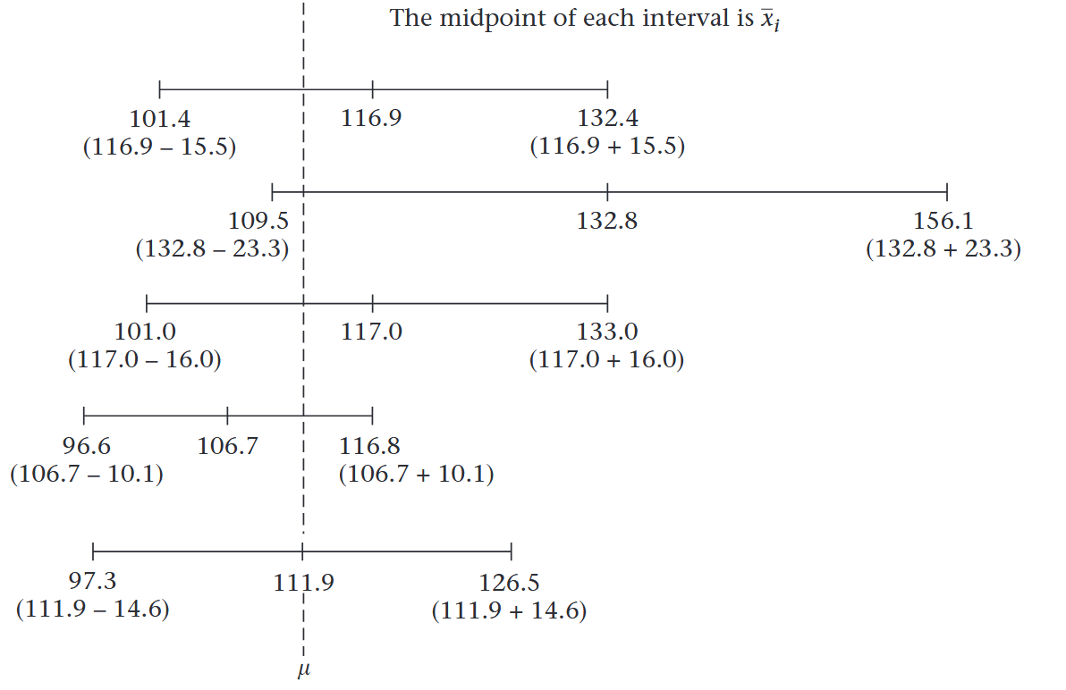
Example: A collection of 95% CIs for the mean $\mu$ as computed from repeated samples of size 10 from the population of birthweights.

The parameter $\mu$ is a fixed unknown constant. How can we state that the probability that it lies within some specific interval is, for example, 95%? The boundaries of the interval depend on the sample mean and sample variance and vary from sample to sample. (see the above picture) Therefore, we cannot say there is a 95% chance that the parameter $\mu$ will fall within a particular 95% CI.

However, we can say the following: Over the collection of all 95% CIs that could be constructed from repeated random samples of size $n$, 95% will contain the parameter $\mu$.

Estimation of the variance of a distribution

In Chapter 2, the sample variance was defined as

$$s^2 = \frac{1}{n-1} \sum_{i=1}^{n} (x_i - \bar{x})^2$$

If our sample $x_1, \dots, x_n$ is considered as coming from some population with mean $\mu$ and variance $\sigma^2$, then how can the unknown population variance $\sigma^2$ be estimated from our sample?

Definition: Let $X_1, \dots, X_n$ be a random sample from some population with mean $\mu$ and variance $\sigma^2$. The sample variance $S^2$ is an unbiased estimator of $\sigma^2$ over all possible random samples of size $n$ that could have been drawn from this population; that is

$$E(S^2) = \sigma^2$$

This statement holds for any underlying distribution.

Chi-square distribution

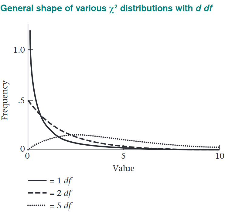
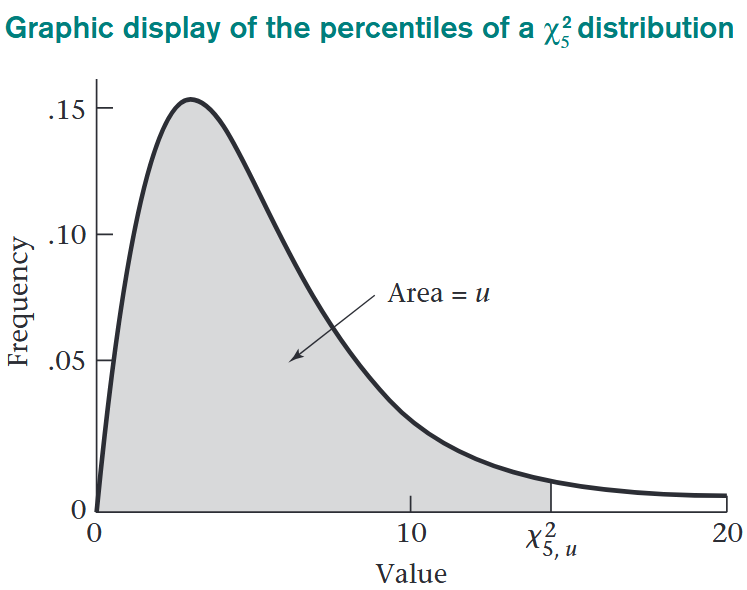
Chi-square distribution: To obtain an interval estimate for $\sigma^2$, chi-square distribution $\chi_i$ are introduced: If $G = \sum_{i=1}^{n} X_i^2$, where $X_1, \dots, X_n \sim N(0,1)$ and the $X_i$'s are independent, then $G$ follows a chi-square distribution with $n$ degrees of freedom ($df$). The distribution is denoted by $\chi_n^2$. NOTE: $X_1, ..., X_n$ must be standard normal distribution. Percentiles of chi-square distribution: The $u$th percentile of a $\chi^2_d$ distribution (i.e., a chi-square distribution with $d df$) is denoted by $\chi^2_{d,u}$, where $P(\chi^2_d < \chi^2_{d,u}) \equiv u$.

Chi-square distribution is a skewed distribution, there is no simple relationship between the upper and lower percentiles.

Interval Estimation

Assume $X_1, \dots, X_n \sim N(\mu,\sigma^2)$, the sampling distribution of $S^2$:

$$S^2 \sim \frac{\sigma^2 \chi^2_{n-1}}{n-1}$$

$Z_i = (X_i - \mu)/\sigma \sim N(0,1)$, then $\sum_{i=1}^{n} Z_i^2 \sim \chi_n^2$:

$$\sum_{i=1}^{n} Z_i^2 = \sum_{i=1}^{n} \frac{(X_i - \mu)^2}{\sigma^2} \sim \chi_n^2 \quad \text{(chi-square distribution with } n \text{ df)}$$

Because we usually don’t know $\mu$, we estimate $\mu$ by $\bar{X}$, there's proof that:

$$\sum_{i=1}^{n} \frac{(X_i - \bar{X})^2}{\sigma^2} \sim \chi_{n-1}^2.$$

Because $(n-1) S^2 = \sum_{i=1}^{n} (X_i - \bar{X})^2$, thus we have

$$\frac{(n-1)S^2}{\sigma^2} \sim \chi^2_{n-1}$$

After rewrite, we have the distribution of sample variance as:

$$S^2 \sim \frac{\sigma^2}{n-1} \chi^2_{n-1}.$$

Interval estimation: A $100\% \times (1 - \alpha)$ CI for $\sigma^2$ is

$$\left[ \frac{(n-1)s^2}{\chi^2_{n-1,\, 1-\alpha/2}},\ \frac{(n-1)s^2}{\chi^2_{n-1,\, \alpha/2}} \right]$$

Derivation: From $S^2 \sim \dfrac{\sigma^2 \chi^2_{n-1}}{n-1}$,

$$P\left( \frac{\sigma^2 \chi^2_{n-1,\, \alpha/2}}{n-1} < S^2 < \frac{\sigma^2 \chi^2_{n-1,\, 1-\alpha/2}}{n-1} \right) = 1 - \alpha$$

Split into two inequalities and solve for $\sigma^2$:

$$\frac{(n-1)S^2}{\chi^2_{n-1,\, 1-\alpha/2}} < \sigma^2 < \frac{(n-1)S^2}{\chi^2_{n-1,\, \alpha/2}}$$

So

$$P\left[ \frac{(n-1)S^2}{\chi^2_{n-1,\, 1-\alpha/2}} < \sigma^2 < \frac{(n-1)S^2}{\chi^2_{n-1,\, \alpha/2}} \right] = 1 - \alpha$$

Replacing $S^2$ with the observed $s^2$ gives the CI above.

A short summary

Interval estimation of mean $\mu$

Let $X_1, \dots, X_n$ be a random sample (independent) from some population with mean $\mu$ and variance $\sigma^2$. For the sample mean $\bar{X} = \frac{1}{n} \sum_{i=1}^{n} X_i$,

$$\begin{aligned} E(\bar{X}) &= \mu \\ \text{Var}(\bar{X}) &= \frac{\sigma^2}{n} \end{aligned}$$

For large $n$, the central-limit theorem for the sample mean gives

$$\bar{X} \dot{\sim} N\left(\mu, \frac{\sigma^2}{n}\right).$$

Interval estimation for the mean $\mu$:

• $\sigma^2$ known: a $100\% \times (1 - \alpha)$ CI is
  $$\left( \bar{x} - z_{1-\alpha/2} \cdot \frac{\sigma}{\sqrt{n}},\ \bar{x} + z_{1-\alpha/2} \cdot \frac{\sigma}{\sqrt{n}} \right)$$
  Shorthand: $\bar{x} \pm z_{1-\alpha/2} \cdot \sigma/\sqrt{n}$. Based on $Z = (\bar{X} - \mu)/(\sigma/\sqrt{n}) \sim N(0,1)$.
• $\sigma^2$ unknown, normal population: if $X_1, \dots, X_n \sim N(\mu, \sigma^2)$, then
  $$\frac{\bar{X} - \mu}{S / \sqrt{n}} \sim t_{n-1}, \text{ $t$ distribution with $(n - 1) df$ }$$
  A $100\% \times (1 - \alpha)$ CI is
  $$\left( \bar{x} - t_{n-1,\, 1-\alpha/2} \cdot \frac{s}{\sqrt{n}},\ \bar{x} + t_{n-1,\, 1-\alpha/2} \cdot \frac{s}{\sqrt{n}} \right)$$
  Shorthand: $\bar{x} \pm t_{n-1,\, 1-\alpha/2} \cdot s/\sqrt{n}$.
• $\sigma^2$ unknown, large sample ($n > 200$): an approximate $100\% \times (1 - \alpha)$ CI is
  $$\left( \bar{x} - z_{1-\alpha/2} \cdot \frac{s}{\sqrt{n}},\ \bar{x} + z_{1-\alpha/2} \cdot \frac{s}{\sqrt{n}} \right)$$
  Shorthand: $\bar{x} \pm z_{1-\alpha/2} \cdot s/\sqrt{n}$.

Interval estimation of variance $\sigma^2$

Let $X_1, \dots, X_n$ be a random sample (independent) from some population with mean $\mu$ and variance $\sigma^2$. For the sample variance $S^2 = \frac{1}{n-1} \sum_{i=1}^{n} (X_i - \bar{X})^2$,

$$E(S^2) = \sigma^2$$

for any underlying distribution; $S^2$ is an unbiased estimator of $\sigma^2$.

Sampling distribution of $S^2$: if $X_1, \dots, X_n \sim N(\mu, \sigma^2)$, normal distribution, then

$$S^2 \sim \frac{\sigma^2}{n-1} \chi^2_{n-1} \quad \text{(chi-square distribution with } n-1 \text{ df)}$$

Equivalently, $(n-1)S^2 / \sigma^2 \sim \chi^2_{n-1}$.

A $100\% \times (1 - \alpha)$ CI for $\sigma^2$ is

$$\left[ \frac{(n-1)s^2}{\chi^2_{n-1,\, 1-\alpha/2}},\ \frac{(n-1)s^2}{\chi^2_{n-1,\, \alpha/2}} \right]$$

This CI requires a normal population. Interval estimates for $\sigma^2$ perform much more poorly than for $\mu$ when the underlying distribution is not normal; use with caution in that case.

Point estimation of a binomial parameter $p$

Example Estimate the prevalence of malignant melanoma in US women aged 45–54. A random sample of $n = 5000$ women is selected; 28 have the disease.

Let $X_i = 1$ if the $i$th woman has the disease, $0$ otherwise (Bernoulli trial with $P(X_i = 1) = p$). Let $X = \sum_{i=1}^{n} X_i$ = number with the disease. Then $X \sim \text{Binomial}(n, p)$, with $E(X) = np$ and $\text{Var}(X) = npq$ ($q = 1 - p$).

The random variable $\hat{p}$ = sample proportion is

$$\hat{p} = \frac{1}{n}\sum_{i=1}^{n} X_i = \frac{X}{n}$$

Since $\hat{p}$ is a sample mean of Bernoulli trials, $E(\hat{p}) = p$; $\hat{p}$ is an unbiased estimator of $p$.

Variance of sample mean: For $X \sim \text{Binomial}(n, p)$,

$$\text{Var}(\hat{p}) = \frac{pq}{n}, \quad se(\hat{p}) = \sqrt{\frac{pq}{n}}$$

In practice, $p$ and $q$ are unknown, so the standard error is estimated by

$$\widehat{se}(\hat{p}) = \sqrt{\frac{\hat{p}\hat{q}}{n}}, \quad \hat{q} = 1 - \hat{p}$$

Interval estimation of $p$

According to central-limit theorem, for larger $n$:

$$\hat{p} \dot{\sim} N\left(p, \frac{pq}{n}\right).$$

Approximate interval estimation : start from

$$P\left(p - z_{1-\alpha/2} \sqrt{\frac{pq}{n}} < \hat{p} < p + z_{1-\alpha/2} \sqrt{\frac{pq}{n}}\right) = 1 - \alpha$$

Split into two inequalities. An exact CI for $p$ would require solving a quadratic in $p$; instead, approximate $\sqrt{pq/n}$ by $\sqrt{\hat{p}\hat{q}/n}$:

$$p - z_{1-\alpha/2} \sqrt{\frac{\hat{p}\hat{q}}{n}} < \hat{p} \quad \text{and} \quad \hat{p} < p + z_{1-\alpha/2} \sqrt{\frac{\hat{p}\hat{q}}{n}}$$

Rearrange to isolate $p$:

$$\hat{p} - z_{1-\alpha/2} \sqrt{\frac{\hat{p}\hat{q}}{n}} < p < \hat{p} + z_{1-\alpha/2} \sqrt{\frac{\hat{p}\hat{q}}{n}}$$

So an approximate $100\% \times (1 - \alpha)$ CI for $p$ is

$$\left( \hat{p} - z_{1-\alpha/2} \sqrt{\frac{\hat{p}\hat{q}}{n}},\ \hat{p} + z_{1-\alpha/2} \sqrt{\frac{\hat{p}\hat{q}}{n}} \right)$$

Shorthand: $\hat{p} \pm z_{1-\alpha/2} \sqrt{\hat{p}\hat{q}/n}$. This method of interval estimation should only be used if $n\hat{p}\hat{q} \geq 5$.

Still need to re read this chapter again.