In a one-sample problem, hypotheses are specified about a single distribution.
In a two-sample problem, two different distributions are compared.
The null hypothesis, denoted by H0, is the hypothesis that is to be tested. The alternative hypothesis, denoted by H1 is the hypothesis that in some sense contradicts the null hypothesis.
Four possible outcomes in hypothesis testing
Truth: H0
Truth: H1
Decision: AcceptH0
H0 is true and H0 is accepted
H1 is true and H0 is accepted (type II error, β)
Decision: RejectH0
H0 is true and H0 is rejected (type I error, α)
H1 is true and H0 is rejected (power, 1−β)
The probability of a type I error is the probability of rejecting the H0 when H0 is true, usually denoted by α and is commonly referred to as the significance level of a test.
The probability of a type II error is the probability of accepting H0 when H1 is true, usually denoted by β.
The power of a test is
1−β=1−The probability of a type II error=P(rejecting H0∣H1 is true)
The general aim in hypothesis testing is to use statistical tests that make α and β as small as possible.
One-sample t test for the mean of a normal distribution: One-Sided Alternatives
Under H0, For random variable (Xˉ−μ0)/(S/n)∼tn−1, thus P(tn−1<tn−1,α)=α.
To test H0:μ=μ0 (σ unknown) vs. H1:μ<μ0 (σ unknown) with a specified significance levelα, compute the value
t=s/nxˉ−μ0
If t<tn−1,α, reject H0. Which means the sample results is extremely rare under H0, less than α, it's unusual.
If t≥tn−1,α, accept H0.
Some concepts
The value t in Equation 7.2 is a test statistic; the test procedure is based on this statistic.
The value tn−1,α is a critical value; if t<tn−1,α, reject H0; if t≥tn−1,α, accept H0.
Computing a test statistic and comparing it with a critical value determined by the type I error is the critical-value method of hypothesis testing.
Traditionally, an α level of exactly .05 is used most frequently.
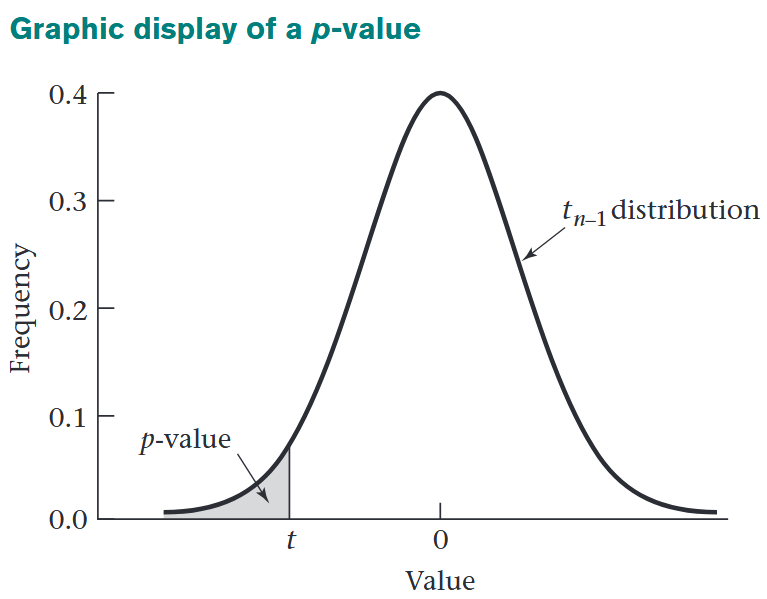
We can also compute p-value: the α level at which the given value of the test statistic (such as t) is on the borderline between the acceptance and rejection regions:
p=P(tn−1≤t)
Thus p is the area to the left of t under a tn−1 distribution.
Given the above formula, The p-value can also be thought of as the probability of obtaining a test statistic as extreme as or more extreme than the actual test statistic obtained, given that the null hypothesis is true.
For the above figure, we know t statistic follows a tn−1 distribution. Hence the probability of obtaining a t statistic that is no larger than the actual t under H0 is P(tn−1≤t)=p-value.
p-value tells us exactly how significant our results are without performing repeated significance tests at different α levels (like α=0.05,0.1,...)
Guidelines for judging the significance of a p-value
If .01≤p<.05, the results are significant.
If .001≤p<.01, the results are highly significant.
If p<.001, the results are very highly significant.
If p>.05, the results are not statistically significant (sometimes denoted NS).
If .05≤p<.10, a trend toward statistical significance is sometimes noted.
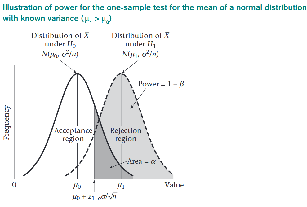
In many situations, we wish to use an alternative hypothesis that μ>μ0,
To test H0:μ=μ0 (σ unknown) vs. H1:μ>μ0 (σ unknown) with significance level α, compute
t=s/nxˉ−μ0
If t>tn−1,1−α, reject H0.
If t≤tn−1,1−α, accept H0.
The p-value is
p=P(tn−1>t)
One-sample t test for the mean of a normal distribution: Two-Sided Alternatives
In the previous section the alternative hypothesis was assumed to be in a specific direction relative to the null hypothesis (μ>μ0 or μ<μ0). In most instances this prior knowledge is unavailable.
A two-tailed test is a test in which the values of the parameter being studied (in this case μ) under the alternative hypothesis are allowed to be either greater than or less than the value of the parameter under the null hypothesis (μ0).
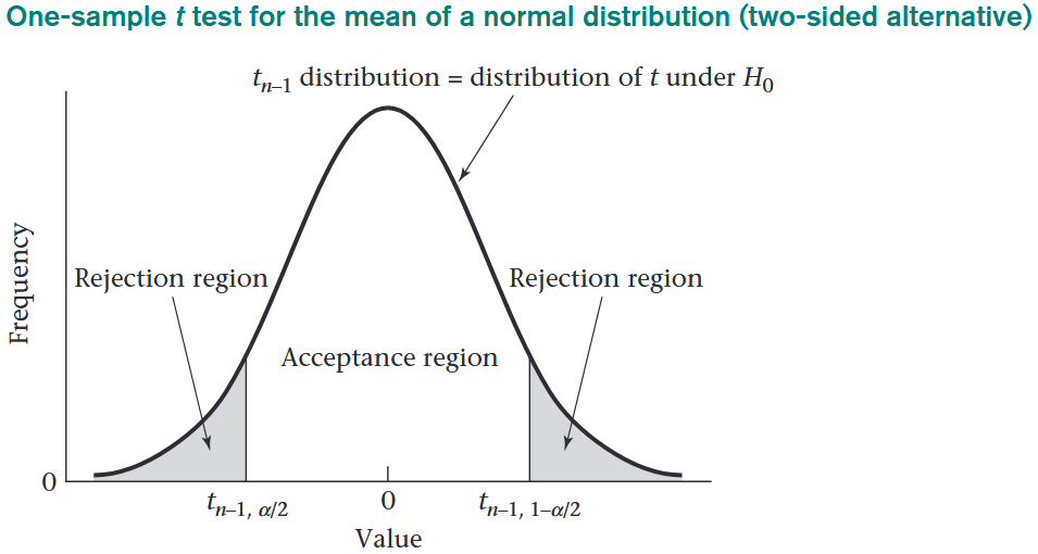
For a two-sided alternative, a reasonable decision rule is to reject H0 if the test statistic t is either too small or too large. That is, reject H0 if t<c1 or t>c2, and accept H0 if c1≤t≤c2.
The constants c1 and c2 are chosen so that the total type I error is α:
For a two-tailed test, half of the type I error is placed in each tail:
P(tn−1<c1∣H0 true)=P(tn−1>c2∣H0 true)=α/2
Under H0,
P(tn−1<tn−1,α/2)=P(tn−1>tn−1,1−α/2)=α/2
Therefore,
c1=tn−1,α/2=−tn−1,1−α/2,c2=tn−1,1−α/2
One-sample t test for a two-sided alternative: to test H0:μ=μ0 vs. H1:μ=μ0 with significance level α, compute
t=s/nxˉ−μ0
If ∣t∣>tn−1,1−α/2, reject H0.
If ∣t∣≤tn−1,1−α/2, accept H0.
Alternatively, we might want to compute a p-value as we did in the one-sided case.
p-value for the two-sided one-sample t test: let
t=s/nxˉ−μ0
Then
p={2P(tn−1≤t),2[1−P(tn−1≤t)],if t≤0if t>0
In words, if t≤0, the p-value is two times the area to the left of t under a tn−1 distribution. If t>0, the p-value is two times the area to the right of t.
For a two-sided alternative, the p-value is the probability under H0 of obtaining a test statistic as extreme as or more extreme than the observed test statistic. Because the alternative is two-sided, extremeness is measured by the absolute value of the test statistic.
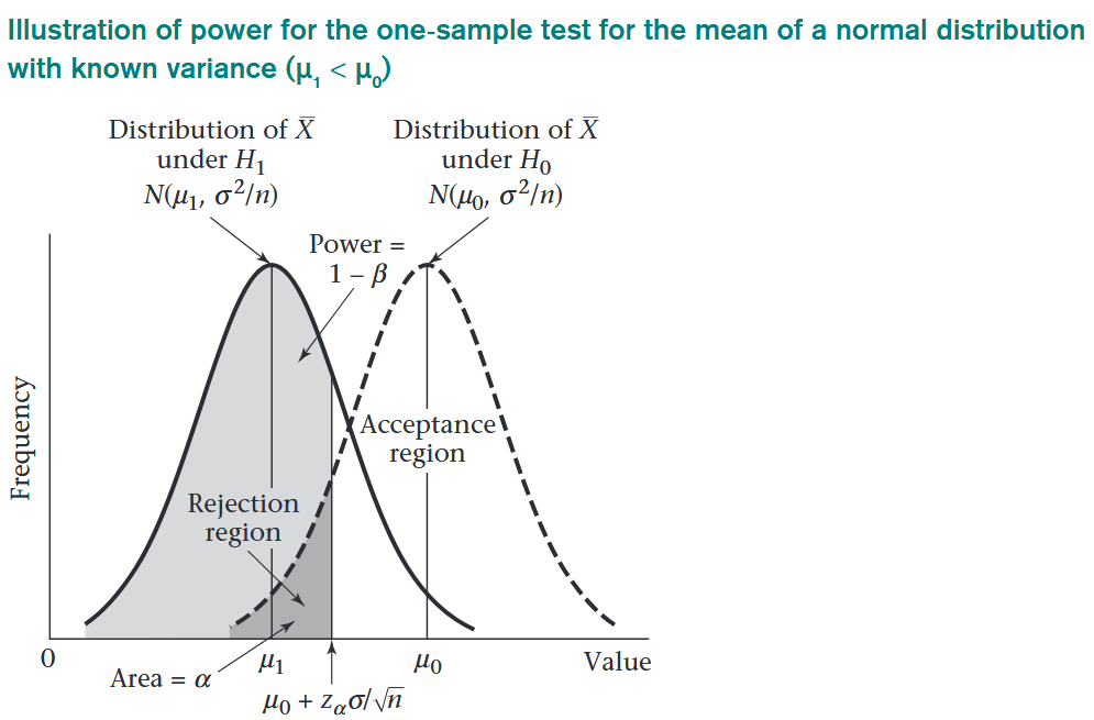
Suppose H0:μ=μ0 vs. H1:μ=μ1. (μ1<μ0)
where the underlying distribution was assumed to be normal and the population variance was assumed to be known.
Under H0,
Z=(Xˉ−μ0)/(σ/n)∼N(0,1)
We can calculate test statistic z, and for a type I error of α, H0 is rejected if z<zα and H0 is accepted if z≥zα.
The power of the test is the probability of rejecting H0 when H1 is true. If the true mean under H1 is μ1, then
Under H1, Xˉ∼N(μ1,nσ2). After standardizing the limit,
Power=Φ(σ/nμ0+zασ/n−μ1)=Φ(zα+σμ0−μ1n)
IMPORTANT: The power of a test tells us how likely it is that a statistically significant difference will be detected based on a finite sample sizen.
If the power is too low, then there is little chance of finding a significant difference and nonsignificant results are likely even if real differences exist between the true mean μ of the group being studied and the null mean μ0.
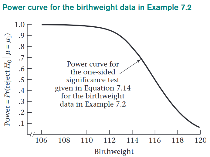
Example: Birthweight data
Compute the power of the test for the birthweight data with an alternative mean of 115 oz and α=.05, assuming the true standard deviation is σ=24 oz.
We have μ0=120 oz, μ1=115 oz, α=.05, σ=24, and n=100. Thus,
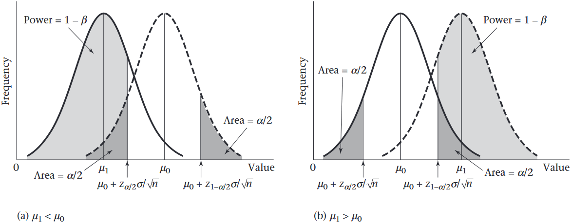
Note: The exact two-sided power formula is more tedious to use than is usually necessary. Specifically, if μ1<μ0, then the second term is usually negligible relative to the first term. However, if μ1>μ0, then the first term is usually negligible relative to the second term. Therefore, the approximate power formula is usually used for a two-sided test because it represents the dominant term in the exact formula.
Illustration of power for a two-sided test for the mean of a normal distribution with known variance
The problem of determining sample size can be summarized as follows: Given that a one-sided significance test will be conducted at level α and that the true alternative mean is expected to be μ1, what sample size is needed to be able to detect a significant difference with probability 1−β? Typical values for the desired power are 80%, 90%, ..., and so forth.
For a one-sided test, we set the desired power equal to 1−β:
Power=Φ(zα+σ∣μ0−μ1∣n)=1−β
We want to solve for n in terms of α, β, ∣μ0−μ1∣, and σ. Since
Φ(z1−β)=1−β
we have
zα+σ∣μ0−μ1∣n=z1−β
Subtract zα from both sides and multiply by σ/∣μ0−μ1∣:
n=∣μ0−μ1∣(−zα+z1−β)σ
Since −zα=z1−α, squaring both sides gives
n=(μ0−μ1)2(z1−α+z1−β)2σ2
Factors affecting the sample size
The sample size increases as σ2 increases.
The sample size increases as the significance level is made smaller (α decreases).
The sample size increases as the required power increases (1−β increases).
The sample size decreases as the absolute distance between the null and alternative means, ∣μ0−μ1∣, increases.
Note: Sample-size estimates are usually only ballpark estimates because μ1 and σ2 are often unknown. These values may be estimated from previous studies, similar experiments, prior knowledge, or a small pilot study. In practice, sample-size calculations are often used to check whether the proposed sample size is reasonably close to what is needed, rather than to determine an exact number.
The one-sided sample-size formula is appropriate when the direction of the alternative mean is specified in advance. If it is not known whether the alternative mean μ1 is greater than or less than the null mean μ0, then a two-sided test is appropriate.
For testing
H0:μ=μ0vs.H1:μ=μ0
with significance level α and desired power 1−β, the sample size needed is
n=(μ0−μ1)2σ2(z1−β+z1−α/2)2
To see this, use the approximate power formula for a two-sided test and solve for n:
Φ(−z1−α/2+σ∣μ0−μ1∣n)=1−β
Since Φ(z1−β)=1−β, we have
−z1−α/2+σ∣μ0−μ1∣n=z1−β
Add z1−α/2 to both sides and multiply by σ/∣μ0−μ1∣:
n=∣μ0−μ1∣(z1−β+z1−α/2)σ
Squaring both sides gives
n=(μ0−μ1)2(z1−β+z1−α/2)2σ2
This required sample size is always larger than the corresponding sample size for a one-sided test, because z1−α/2>z1−α.
Sometimes the treatment effect is already believed to exist, so the main goal is not hypothesis testing but estimating the effect with a desired degree of precision. In this case, sample size can be chosen based on the desired width of a confidence interval.
Example: Cardiology
Suppose propranolol is known to lower heart rate over 48 hours in patients with angina at standard dosage levels. A new study uses a higher dose, and investigators want to estimate the drop in heart rate with high precision.
If precision is measured by the width of a two-sided 100(1−α)% confidence interval, then the CI for the true mean decline μ is
xˉ±tn−1,1−α/2ns
The width of this interval is
2tn−1,1−α/2ns
If we want the CI width to be no wider than L, then
2tn−1,1−α/2ns=L
so
n=L24tn−1,1−α/22s2
Because tn−1,1−α/2 is often approximated by z1−α/2, the required sample size is approximately
n=L24z1−α/22s2
Example: Cardiology
Find the minimum sample size needed to estimate the change in heart rate μ if the two-sided 95% CI for μ must be no wider than 5 beats per minute and the sample standard deviation for change in heart rate is s=10 beats per minute.
We have α=.05, s=10, and L=5. Therefore,
n=(5)24z.9752(10)2=254(1.96)2(100)=61.5
Thus, at least 62 patients need to be studied.
The Relationship Between Hypothesis Testing and Confidence Intervals
H0 is rejected if and only if the two-sided 100(1−α)% confidence interval for μdoes not containμ0.
H0 is accepted if and only if the two-sided 100(1−α)% confidence interval for μdoes containμ0.
Note: The hypothesis-testing approach and the confidence-interval approach often lead to the same conclusion, but they emphasize different information. A p-value tells us how statistically significant the result is, while a confidence interval shows the likely range of the parameter and helps judge the practical size of the effect. Therefore, it is good practice to report both the p-value and the confidence interval whenever possible.
Example: Cardiovascular Disease
For the cholesterol data, the p-value of .037 tells us how statistically significant the result is. The 95% confidence interval for μ, (173.58,189.46), gives a range of likely values that μ might assume. These two types of information are complementary.
 For the above figure, we know statistic follows a distribution. Hence the probability of obtaining a statistic that is no larger than the actual under is -value.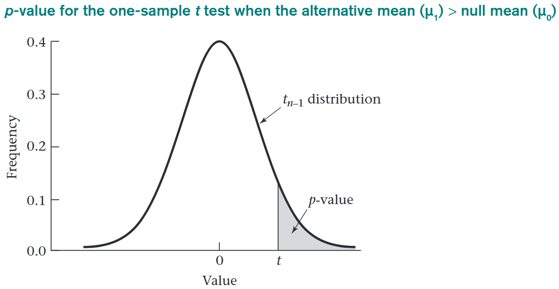
 Alternatively, we might want to compute a -value as we did in the one-sided case.